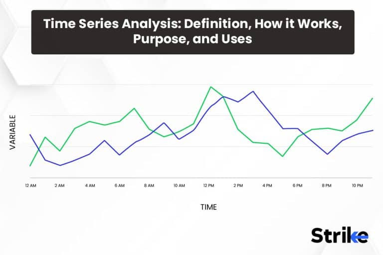
Time Series Analysis: Definition, How it Works, Purpose, and Uses

Time series analysis is a statistical technique used to model and explore patterns in data recorded sequentially over time.

Time series analysis practitioners first visualize time series data to identify trends, seasonality and other patterns before selecting suitable modeling techniques. Common approaches include autoregressive, moving average and ARIMA modeling which quantify relationships between past and current values. Forecasting methods then generate predictions for future time points.

The goal of time series analysis is four-fold: to make valuable predictions, explain what drives observed changes, identify cycles and durations, and monitor for anomalies. Key advantages include the ability to detect trends, quantify relationships, handle non-stationarity, and filter noise. Example application domains span various industries and sciences and encompass tasks like sales forecasting, weather prediction, anomaly detection in manufacturing, and econometric modeling of national indicators. The diversity of use cases demonstrates the wide practical utility of time series analysis.

What is Time Series Analysis?

Time series analysis is a statistical technique that analyzes data recorded over time, typically at successive equally spaced points in time. Time series’ goal is to carefully study the past patterns in the data to make meaningful future predictions. Time series data have a natural ordered sequence over time and the data points are usually successive measurements made over an evenly spaced time interval. Examples of time series data include daily stock prices, monthly sales figures, yearly temperature readings, etc.

Time series analysis techniques are divided into two broad categories – time domain and frequency domain. Time domain techniques use direct observations of the data as it evolves over time. For example, plotting the time series on a graph reveals ups and downs and cyclic movements that are analyzed. Statistical techniques like moving averages smooth out short-term fluctuations to reveal longer-term trends and cycles. Autocorrelation analyzes correlations between successive observations at different time lags. Frequency domain techniques like Fourier transforms decompose the overall variations of a time series into distinct cyclical components of different frequencies. 

Time series often exhibit long-term increases or decreases over time. For example, sales steadily grow over several years. Trend analysis helps identify and predict long-term movements.

Time series often show recurrent short-term cycles such as higher retail sales around holidays. Seasonal adjustment removes these fluctuations to reveal underlying trends.

Time series contain random disturbances that add variability. Smoothing techniques filter out noise to uncover patterns.

Many time series techniques require stationarity, which means statistical properties like mean and variance are constant over time. Differencing and transformations stabilizes the time series.

Successive observations in time series data are usually interdependent. Autocorrelation quantifies these relationships and incorporates dependence into models.

Time series analysis has applications in many fields including economics, finance, geology, meteorology, and more. It is useful for forecasting, tracking trends, detecting seasonality, understanding cyclic behavior, and recognizing the relationship between variables. Overall, time series analysis is a crucial statistical tool for making data-driven predictions by learning from historical observations taken sequentially through time.

What are the components of Time Series Analysis?

Time series analysis includes six main components, including data preparation, exploratory data analysis, model identification, etc.

1. Data Preparation

Data Preparation is the first and crucial step of any time series analysis. It involves collecting the relevant historical time series data, checking for completeness and accuracy. Any missing values or outliers need to be addressed during this stage. The data is also measured for stationarity which is an important assumption in time series modeling. Appropriate transformations may be applied to make the data stationary if needed.

2. Exploratory Data Analysis

The next step involves Exploratory Data Analysis which helps gain initial insights into the patterns and characteristics of the data. Statistical techniques are used to analyze the trends, seasonality, correlations and cyclical behavior present in the data. Plotting tools like time series plots, autocorrelation function and partial autocorrelation function graphs are widely used to examine these underlying components at a preliminary level. Any unusual observations or anomalies are also noted at this stage.

3. Model Identification 

After understanding the properties of data, the next step is Model Identification which involves selecting the most suitable forecasting model. Different model types like AR, MA, ARMA, ARIMA or SARIMA are tested based on the patterns observed during exploratory analysis. Model identification also determines the required number of terms and lag structure. Statistical tests help select the best fitting candidate model.

4. Model Forecasting

Once identified, the selected model is used for Model Forecasting where future values of the time series are predicted. The identified model is applied on the historical data to forecast one or multiple time periods ahead. Key evaluation metrics analyze the forecast accuracy on test data sets. If required, additional variables may also be included to improve the forecast.

5. Model Maintenance

Model Maintenance involves monitoring the model performance over time. As new actual observations become available, the model needs periodic re-evaluation and updating if required. This ensures the selected model continues providing reliable forecasts with changing behaviors and environments over time.

6. Application Domains

Finally, the learned concepts and developed models can be applied across various application domains that exhibit time dependency. Examples include demand forecasting, sales prediction, predicting disease outbreaks, stock market trend analysis and more.

The diversity of application areas highlights the wide utility of time series analysis across many scientific and business disciplines. However, domain knowledge is critical in constructing useful models tailored to the specifics of each field.

How Does Time Series Analysis Work?

Time series analysis works by applying statistical methods to data observed and recorded over uniform time intervals. The goal is to uncover meaningful patterns, build explanatory models, and generate forecasts. 

Data Collection

The first step is gathering observations over evenly spaced intervals of time. The spacing between observations is called the sampling frequency. Common frequencies include yearly, quarterly, monthly, weekly, daily, and hourly. The sampling should be consistent over the entire time span of interest. Any missing values must be handled by interpolation or imputation methods.

Exploratory Analysis 

Once the time series dataset is assembled, initial insights are obtained by visualizing the data with plots. A simple time series plot with the observations on the y-axis and time on the x-axis reveals important qualities like trends, spikes, seasonal cycles, and anomalies. Statistical summaries like the mean, variance, autocorrelations and spectral density provide additional diagnostic information. The goal is to characterize key data properties prior to modeling.

Real-world time series often exhibit non-stationarity – where the mean, variance and autocorrelations change over time. Many forecasting methods work best on stationary data. Thus, mathematical data transformations are sometimes applied to convert a non-stationary series to a stationary one. Common techniques include smoothing, detrending, differencing, and removing seasonal or cyclical components.

Based on the exploratory analysis, an appropriate time series model is selected. Common model types include autoregressive models, moving average models, ARIMA models, regression models, and neural networks. The model choice is based on both data characteristics and domain knowledge about the underlying data generating process. Model parameters are estimated from the data, often using methods like ordinary least squares. 

The fitted model is checked to ensure it meets required assumptions and has a good fit. Residual analysis, prediction errors, and information criteria are used to validate model adequacy. Once a suitable level of performance is attained, the model specification is revised and the parameters are re-estimated if diagnostics show any shortcomings.

With a validated model, forecasts are produced. In-sample forecasts are generated on the historical dataset used for fitting the model. Out-of-sample forecasts apply the model to predict future values beyond the estimation dataset. Point forecasts give the most likely prediction, while interval forecasts provide a range of probable values. As new data arrives, forecasts are updated by re-estimating the model parameters. 

To keep forecasts accurate over time, the models need ongoing maintenance. This includes monitoring prediction errors to check for deterioration in model performance. Structural change detection methods identify if the underlying data patterns have shifted, indicating a model update is required. Ensemble forecasts from multiple models often provide robustness.

How are Graphs and Charts used in Time Series Analysis?

Visualizing time series data through graphs and charts is an essential first step in any time series analysis. Time series plots reveal important characteristics of the data like trends, seasonal patterns, outliers and structural breaks. Before applying statistical models, visualization provides exploratory insights and guides subsequent analysis. 

The most common time series graph is a time series plot with the observations on the y-axis and time on the x-axis. 

Connecting successive observations with a line highlights the evolution of the series over time. A smoothed or moving average line overlaid on the raw data highlights longer-term patterns by filtering short-term fluctuations. Plotting transformations like logarithms and differencing reveals types of non-stationarity like changing variability. 

Scatter plots show correlations between two time series and lag plots display autocorrelations at various lags. Cross-correlation plots quantify leads and lags between series. A correlogram compactly visualizes autocorrelations for multiple lags.

Spectral plots depict the frequency composition of a series. Dominant periodicities and seasonal cycles appear as peaks in the spectral density. Periodograms estimate the spectrum from the raw data.

For economic time series, charts illustrating annual/quarterly growth rates, cyclical components, and trends aid decomposition into underlying components. Plotting accelerations reveals turning points associated with recessions.

Univariate distributions of raw values, returns, or forecast errors summarized through histograms, density plots, normal quantile plots assess distributional assumptions needed for forecast intervals. 

Heatmaps and contour plots depict time-varying patterns in matrix data like volatilities, correlations and covariances. Cluster heatmaps identify groups of related series.

Heatmaps are used extensively by traders and investors to find favorable opportunities out of a specific group or sectors. There are a number of scanners available on the internet that fetch heatmaps under specified sectors or groups. An example of such a scanner is added below. 

The image uploaded above is achieved from Strike.money. The specific heatmaps module will scan through the thousands of stocks and create specified heatmaps under selected indices or sectors as one can observe in the above image.

The strike.money scanner also scans and produces heatmaps based on Price, RSI, MFI, Stochastic, % away from 52Wk high/low, % away from 200, 100, 50 SMA. 

This is exceptionally useful to traders selecting stocks based on certain criterias. 

The visualized raw data guides fitting an appropriate time series model. Scatter plots of residuals check model adequacy. Recursive forecasts retrospectively show if models capture turning points. Distribution plots verify forecast intervals. 

What is the purpose of Time Series Analysis?

The main purpose of time series analysis is to extract useful information from time-dependent data and gain insights into the underlying patterns, relations and trends. It helps identify the evolutionary behavior of a variable over regular intervals of time. Time series analysis aids in forecasting future values based on historical observations. By developing statistical models that capture seasonality, trend and noise components through decomposition techniques, it becomes possible to predict where a series is headed in the coming periods. This supports decision making processes for inventory management, production planning, demand projections and resource allocation.

It also reveals insights into cyclical fluctuations and pinpoints phases of peaks, troughs and other transitions. This understanding helps assess the impacts of external factors on a measured phenomenon over sequent time periods. Time series models further detect auto-correlations that exist within a single time series due to its own interactions and interdependencies over multiple past instances. The outputs assist in risk analysis and generating accurate forecasts. Overall, time series analysis aims to describe, model and project patterns in dynamic systems varying with time.

What are the Types of Time Series Analysis?

Time series analysis types of different statistical models and techniques to uncover patterns, understand structure, and make predictions using temporal data. The following eleven are the main categories of time series analysis.

1. Regression Models

Relate the time series to other explanatory variables like economic factors, prices, or demographics. Linear regression is most common, but nonlinear relationships are also sometimes modeled. Useful for quantifying causal effects.

2. Autoregressive Models 

Predict future values using a weighted sum of past observations plus an error term. Model the autocorrelation inherent in time series. ARIMA models are a very popular example.

3. Smoothing Models

Use weighted averaging of past observations to smooth out noise and highlight trends and seasonality. Includes simple, exponential, and state space smoothing methods.

4. Machine Learning Models

Modern techniques like artificial neural networks, random forests, and gradient boosting machines have been adapted to handle time series data and make highly flexible predictions.

5. State Space Models 

Represent time series using latent state variables that evolve over time. Allows modeling complex dynamics through multicomponent state vectors.

6. Gaussian Processes 

A flexible nonparametric Bayesian approach to time series modeling. Utilises kernel functions to model correlations between time points.

7. Spectral Analysis

Decompose a time series into underlying cyclical components of different frequencies using Fourier and wavelet transforms. Reveals periodicities. 

8. Threshold Models

Allow different data generating processes and model parameters to apply before and after threshold values are crossed. Capture structural breaks.

9. Markov Models

Model transitions between a series of possible states over time as a Markov process. The next state depends only on the current state.

10. Hidden Markov Models

Expand Markov models by assuming the states are hidden. Use only the observable time series to estimate state sequences and transition probabilities. 

11. Archetype Analysis

Identify recurrent archetypal patterns in the time series using basis functions from a dictionary of archetypes. Concise lower dimensional representation.

Many types of time series models have emerged from statistics, econometrics, signal processing, and machine learning. Linear models like ARIMA are simple and interpretable. Machine learning provides highly flexible nonlinear modelling. State space and Bayesian models incorporate sophisticated dynamics. The diversity of techniques provides a toolkit to tackle different types of temporal data problems.

What are the Advantages of Time Series Analysis?

Time series analysis provides 11 main advantages when modeling temporal data. The eleven most significant advantages include the following.

1. Making Predictions

Time series models such as ARIMA and exponential smoothing produce forecasts for future values in the series. This supports planning, goal-setting, budgeting and decision-making. Prediction intervals also quantify forecast reliability.

2. Understanding Drivers

Time series modeling yields insight into the underlying components and variables that drive observed changes over time. This explanatory power reveals why and how a process behaves.

3. Quantifying Relationships

Statistical measures like autocorrelation and cross-correlation quantify the relationships between observations in time series data. Regression modeling estimates causal relationships with other variables. This enables hypothesis testing.

4. Handling Nonlinearity

Sophisticated machine learning algorithms model complex nonlinear relationships hidden in time series data that cannot be captured by simple linear models.

5. Modeling Trends

Time series models effectively detect and characterize trends found in data, even amongst a high degree of noise and variability. This aids long-term thinking.

6. Modeling Cycles

Analysis techniques like spectral decomposition extract short-term, medium-term and long-term cyclical patterns occurring in time series. This finds recurring periodicities.

7. Estimating Seasonality 

Seasonal decomposition, differencing, and modelling techniques sometimes estimate, forecast and adjust for regular seasonal fluctuations. This improves forecasting.

8. Filtering Noise

Smoothing methods reduce noise and randomness to uncover the stable underlying time series components and relationships. The signal becomes clearer.

9. Handling Missing Data

Time series methods such as imputation and state space models estimate missing observations and interpolate gaps by exploiting temporal correlations.

10. Detecting Anomalies

Changed behavior, level shifts, outliers and anomalous patterns are sometimes detected using time series monitoring, process control charts and intervention analysis.

11. Comparing Series

Measures like cross-correlation, dynamic time warping, and similarity clustering allow comparing and aligning different time series to identify shared behaviors.

Time series analysis provides a toolbox of techniques to transform raw temporal data into actionable insights. Key advantages include making skillful predictions, deeper understanding, quantifying relationships, modeling complexity, trend/cycle analysis, denoising data, handling missing values, and detecting anomalies.

What are the Disadvantages of Time Series Analysis?

Even though time series analysis has numerous advantages, there are eleven drawbacks, restrictions, and disadvantages that should be taken into account.

1. Data Dependence

Time series models require sufficient historical data to train and validate. Performance suffers with short time series or small sample sizes. Data must adequately represent all important patterns.

2. Assumption Dependence 

Simple linear models like ARIMA rely on assumptions of stationarity, normality, homoscedasticity, etc. Violations undermine reliability. Machine learning models have fewer strict assumptions.

3. Overfitting

Complex models with excessive parameters tend to overfit training data, limiting generalizability. Regularization, cross-validation and parsimony help prevent overfitting.

4. Nonstationarity

Time series data is often nonstationary. Transformations to stabilize the mean and variance add complexity. Models sometimes fail if nonstationarity is undetected.

5. Expense

Large time series datasets require significant data storage capacity. Advanced analytics, forecasting software, and technical skills add cost. Lack of expertise limits value.

6. Maintenance

Time series models require ongoing monitoring and re-estimation to keep them aligned with changing data patterns. Ignoring model degradation impacts accuracy over time.

7. Spurious Relationships 

Correlation does not imply causation. Regressions at times uncover false associations unrelated to true causal effects due to confounding factors.

8. Unpredictable Shocks 

Major unexpected exogenous events sometimes cause structural breaks in historical patterns, ruining forecasts. Black swan events are difficult to model.

9. Simplifying Assumptions

Mathematical tractability requires simplifying complex real-world phenomena into statistical models. This abstraction loses nuance and introduces uncertainty.

10. Temporal Misalignment

Comparing time series requires aligning them temporally using methods like dynamic time warping. Misalignment degrades accuracy.

11. Technical Complexity

Many advanced time series techniques require specialized mathematical/statistical expertise. Simple methods sometimes suffice for basic forecasting tasks.

Time series analysis has some inherent challenges and drawbacks. No single technique dominates – multiple methods are often required to address different data needs and limitations. Thoughtful analytic design, caution against over-interpretation, and model robustness checks mitigate these disadvantages.

How to use Time Series Analysis?

Time series analysis provides a valuable set of methods for modeling data collected sequentially over time. Here are twelve key steps for effectively applying time series analysis.

Specify the Problem 

Clearly articulate the analytical goals and questions before collecting data. This focuses the analysis and metrics. Common goals include forecasting, trend analysis, causal impact estimation, pattern detection, etc.

Gather Time Series Data

Obtain measurements over evenly-spaced time intervals covering an adequate period to represent all important patterns. Daily, weekly, monthly, quarterly, and yearly time scales are common.

Clean and Prepare Data

Inspect for anomalies and missing data. Perform preprocessing tasks like smoothing, interpolation, outlier removal, and data transformations to stabilize the series.

Visualise Patterns

Create time series plots to inspect overall patterns, long-term trends, variability, seasonality, structural changes and anomalies. Visual clues guide analysis.

Check Stationarity 

Assess stationarity via statistical tests and plots. Transform non stationary data to stabilize the mean and variance over time, if needed. Log or power transforms are common.

Measure Dependency

Quantify the autocorrelation at various lags using correlograms. High autocorrelation violates independence assumptions and influences model selection. 

Decompose Components

Isolate trend, seasonal, cyclical and noise components through smoothing, seasonal adjustment, and spectral analysis. Model components separately.

Build Models

Identify candidate time series models based on visualized patterns and theoretical assumptions. Assess fit on training data. Avoid overfitting out-of-sample. 

Make Forecasts

Use the fitted model to forecast future points and horizons. Calculate prediction intervals to quantify uncertainty.

Validate Models

Evaluate in-sample goodness-of-fit and out-of-sample forecast accuracy. Check residuals for independence and normality. Refine as needed.

Monitor Performance

Continually track forecasts against actuals and update models to account for changing data dynamics. Don’t ignore degradation.

Choose Parsimonious Models

Prefer simpler time series models over complex alternatives, if performance is comparable. Beware overfitting complex models to noise.

Thoughtful time series analysis moves through key phases of problem definition, data preparation, exploratory analysis, modeling, prediction, validation and monitoring. Understanding time dependent data patterns drives effective application and interpretation of analytical results.

How is Time Series used in Trading?

Time series analysis is extensively used in financial trading strategies and algorithms. Historical price data for assets like stocks, futures, currencies and cryptocurrencies exhibit patterns that inform profitable trades. Traders employ time series models for forecasting, risk analysis, portfolio optimization and trade execution.

Price forecasting is key for speculating on future direction. Models like ARIMA are fitted on historical bars to predict next period prices or price changes. Technical indicators derived from time series like moving averages generate trade signals. Machine learning classifiers categorize patterns preceding price increases or decreases. These forecasts trigger entries and exits. 

Volatility modeling analyzes the variability of returns. GARCH models the volatility clustering observed in asset returns. Stochastic volatility models the latent volatility as a random process. Volatility forecasts optimize position sizing and risk management.

Cycle analysis detects periodic patterns across multiple timescales from minutes to months. Fourier analysis and wavelets quantify cycles. Combining cycles into composite signals provides trade timing. Cycles assist in entries, exits and profit taking.

backtesting evaluates strategy performance by simulating trades on historical data. Trading systems are developed iteratively by assessing past hypothetical performance. Statistical rigor validates if observed returns exceed reasonable risk thresholds.

Model validation techniques like walk forward analysis partition past data into in-sample fitting and out-of-sample testing periods. This avoids overfitting and checks for robustness.

Correlation analysis quantifies which instruments move together. Pairs trading strategies exploit temporary divergences between correlated assets. High correlation allows hedging and risk reduction.

Feature engineering extracts informative input variables for models from raw price data. Lagged prices, technical indicators, transformed series and macroeconomic data become model inputs.

Is Time Series Analysis used to predict stock prices?

Yes, time series analysis is commonly used to predict and forecast future stock prices. However, there are some important caveats to consider regarding the challenges of accurately modeling financial time series data.

Time series methods like ARIMA and GARCH models have been applied to stock prices for short-term forecasting and volatility prediction. These quantify historical autocorrelations in returns. Machine learning techniques also show promise modeling complex stock price patterns. 

In-sample model fit to past data is often strong. However, out-of-sample accuracy degrades quickly as the forecast horizon extends farther into the uncertain future. Stock prices follow random walk patterns according to efficient market theory, limiting predictability.

Unexpected news events, economic forces, investor behavior shifts and other exogenous factors sometimes suddenly alter established price patterns. This causes structural breaks that invalidate statistical models derived from historical data.

High volatility with frequent large price spikes make stock prices challenging to predict compared to smoother time series. Nonstationarity requires transformations but distributions often remain non-normal.

Spurious correlations and overfitting in-sample are risks if models lack causative explanatory variables. Correlation does not guarantee reliable out-of-sample forecasts. Simplicity avoids overfitting.

Trading frictions like spreads, commissions and slippage erode profitability of minor predictable price movements. Large price swings are needed for profitable trading but large swings are inherently less predictable.

Is Time Series Analysis effective in forecasting stock prices?

Yes, time series analysis is widely used to forecast stock prices. However, its effectiveness has limits.

Time series models are able to make short-term stock price forecasts by extrapolating historical patterns into the future. Methods like ARIMA and exponential smoothing applied to daily closing prices predict the next day’s price or price change. Technical analysis indicators built from time series like moving averages also aim to forecast future movements.

Machine learning algorithms utilizing time series data as inputs have also demonstrated an ability to make profitable stock price predictions in some cases. Deep learning methods like LSTM neural networks sometimes model complex nonlinear patterns. Models also incorporate other predictive variables like fundamentals, news sentiment, or technical indicators.

However, the inherent unpredictability and efficient market assumptions around stock prices constrain forecasting performance. Time series models make predictions based on historical correlations continuing into the future. But new events and information that alter investor behavior rapidly invalidate observed patterns. This limits how far forward historical extrapolations remain relevant.

In very liquid stocks, arbitrage activity quickly eliminates any predictable patterns that models learn. This efficient market hypothesis means consistent excess returns are difficult to achieve simply from data-driven forecasts. Spurious patterns often arise just from randomness rather than genuine information.

Time series models sometimes only have a predictive edge in less efficient market segments with lower trading volumes. But even there, structural changes in market dynamics sometimes still render patterns obsolete.

For longer term forecasts, fundamental valuation factors and earnings expectations rather than technical time series tend to dominate stock price movements. Time series has more relevance for higher frequency price changes over short horizons of days to weeks.

How can Time Series Analysis and Moving Average work together?

Time series analysis and moving averages work together symbiotically to better understand and forecast temporal data. 

Moving averages smooth out short-term fluctuations in time series data to highlight longer-term trends and cycles. They act as low pass filters to remove high frequency noise. Different moving average window lengths filter different components.

Visual inspection of moving averages layered over raw time series on line charts offers a quick way to visually identify overall trends, local cycles, and potential turning points. The crossover of short and long moving averages is a simple trading indicator. 

Moving averages quantify local means at each point in the time series. Measuring the difference between the series and its moving averages isolates short and long-term components. This decomposition aids modeling.

Calculating the autocorrelation of moving averages rather than raw observations removes noise and stabilizes the time series. This improves the fit of autoregressive models like ARIMA that assume stationarity.

Incorporating moving averages directly as input variables or components within autoregressive and machine learning models provides useful smoothed explanatory features. The models learn to make predictions based partially on the moving average signals.

Testing different moving average window lengths for optimal predictive performance through validation guides selection of the most useful smoothing parameters for a given time series and forecast horizon.

Synthesizing multiple moving averages rather than relying only on a single smoothed series better adapts to shifts in the underlying data-generating process over time. Combining signals improves robustness.

Can Time Series Analysis be Used with Exponential Moving Average?

Yes, time series analysis is effectively combined with exponential moving averages (EMA). 

Exponential moving averages apply weighting factors that decrease exponentially with time. This gives greater influence to more recent observations compared to simple moving averages.

EMAs serve as smoothing filters that preprocess a noisy raw time series. The smoothed EMA series reveals slower-moving components like trends and cycles that are useful predictors in time series forecasting models. 

An EMA also provides a flexible localized approximation of the time series. The level and slope of the EMA at a given point provides a summary of the local trend and level. Time series models incorporate EMA values and gradients as explanatory variables.

The difference between the original series and its EMA filters out short-term fluctuations. Modeling this residual series improves volatility and variance forecasts since much of the ephemeral noise gets removed.

EMAs are embedded in exponential smoothing methods for time series forecasting. Simple exponential smoothing applies an EMA to the series with an adaptive weighting parameter. More advanced exponential smoothing extends this to trended and seasonal data. The EMA inherently features in these models.

Crossovers of short and long window EMAs produce trade signals on momentum shifts. These indicators complement statistical model forecasts with empirical rules for market entry and exit timing. 

Comparing model predictions to EMA benchmarks helps diagnose when models are underperforming. Divergences flag structural changes in the data requiring model retraining. The EMA reference also guards against overfitting.

What are Examples of Time Series Analysis data?

Here are seven examples of time series data commonly analyzed with statistical and machine learning models.

Stock Prices

Daily closing prices of a stock over many years forms a time series. Price fluctuations reflect market forces. Analysts look for trends, volatility, seasonality, and predictive signals. Time series models forecast future prices.

Sales Figures

Monthly sales totals for a company comprise a time series. Sales exhibit seasonal patterns, trends, and business cycles. Time series decomposition isolates components while ARIMA models forecast future sales.

Weather Recordings 

Measurements of temperature, rainfall, or wind speed captured on a regular time interval. Weather data shows seasonality and longer climate cycles. Time series methods detect patterns and predict weather.

Economic Indicators

Key metrics like GDP, unemployment, manufacturing activity, consumer confidence, inflation, and interest rates tracked over years or decades reveal economic growth, recessions, and booms. Regression analysis relates indicators.

Web Traffic

The number of daily or hourly website visitors forms a time series that quantifies popularity. Trends, seasons, events, and news cause variations. Anomaly detection identifies unusual changes.

Sensor Readings

Time series from internet of things sensors like temperature, pressure, power consumption, or vibration. Sensor data is analyzed to monitor equipment health, detect anomalies, and predict failures. 

Audio Signals

Sound waveform samples over time comprising music, speech, or noise. Audio time series analysis involves filtering, spectral analysis, and digital signal processing for compression or features.

Analyzed time series can be stationary or nonstationary, cyclic, seasonal, noisy, intermittent, and irregular. Any phenomenon measured sequentially over uniform time intervals constitutes a time series. The diversity of examples highlights the broad applicability of time series modeling techniques.

Is Time Series Analysis Hard?

Time series analysis has a reputation for being a challenging field, but the difficulty depends greatly on context and the methods used.

Yes, some of the more advanced statistical techniques like ARIMA, vector autoregression, and state space models require mathematical knowledge and experience to apply and interpret correctly. However, simpler forecasting methods and visual analysis suffice for many applications.

The theory supporting complex time series modeling is intellectually demanding. But modern software packages automate many complex calculations and diagnostics. This reduces the practical challenge of application, if proper caution is exercised.

Nonstationary, noisy data with multiple seasonal cycles poses difficulties. But transforming and decomposing time series into more tractable components simplifies analysis. Treating each piece wisely reduces overall complexity. 

 Trading applications face added challenges of low signal-to-noise ratios, non-normal distributions, and structural breaks. Reasonable expectations and combining quantitative models with human insight keep trading viable.

Is Time Series Analysis Quantitative?

Yes, time series analysis is a quantitative discipline involving statistical modeling and mathematical techniques.

Time series analysis relies heavily on quantitative methods from statistics, econometrics, signal processing, and machine learning. Comprehending and applying time series requires comfort with statistical reasoning and mathematical thinking.

Exploratory analysis involves quantitative techniques like autocorrelation, spectral decomposition, stationarity tests, and variance stabilization transforms. Appropriate modeling requires selecting mathematically formulated model classes like ARIMA, state space models, or VAR processes. 

Fitting time series models involves quantitative estimation methods like regression, maximum likelihood estimation, Bayesian inference, or numerical nonlinear optimization. Model adequacy is assessed using quantitative diagnostic checks on residuals, information criteria, and prediction errors. 

Forecasting processes need quantification of uncertainty through numeric metrics like mean squared error, interval widths, empirical prediction distributions, and quantile loss. Model selection and comparison requires numerical evaluation metrics.

Time series outputs including point forecasts, prediction intervals, probabilistic forecasts, and quantified model uncertainties enable data-driven decision making. But interpreting their meaning and limitations correctly depends on statistical literacy.

Domain expertise and qualitative context remain essential for useful applicability. But the underlying techniques for processing, modeling, forecasting, and decision making from time series data are fundamentally quantitative. Even basic visualizations like time series plots depend on quantitative axes and numerical summaries.

Time series analysis is a quantitative discipline reliant on mathematical and statistical competency. It leverages numerical techniques to extract patterns, insights and forecasts from data ordered over time. The quantitative orientations complement the qualitative perspectives from domain knowledge for impactful time series modeling.

What is the difference between Time Series Analysis and Cross-Sectional Analysis?

Here is an overview of the key differences between time series analysis and cross-sectional analysis.

Time Series Analysis

• Studies observations recorded sequentially over time for a single entity or process.
• Observations are temporally ordered and spaced at uniform time intervals.
• Models temporal dependencies like trends, autocorrelation, cyclical patterns.
• Commonly used for forecasting future values.

Cross-Sectional Analysis

• Studies observations recorded across multiple entities or subjects at a single point in time.
• Observations are for different subjects rather than timed observations of one subject.
• Models relationships between variables observed on the same subject.
• Used to determine correlation and causality between variables.

Other Differences

• Time series data has a natural ordering that cross-sectional data lacks.
• Time series is prone to autocorrelation while cross-sectional errors are independent.
• Time series sometimes exhibit non-stationarity whereas cross-sectional data is stationary.
• Time series models extrapolate patterns over time, cross-sectional models interrelate explanatory variables.
• Time series analysis aims to forecast, cross-sectional analysis aims to infer causal relationships.
• Time series has temporal dependencies, cross-sectional analysis studies spatial relationships.

Time series analysis focuses on sequential data over time while cross-sectional analysis studies data across multiple subjects simultaneously. Their domains, assumptions, methods and objectives differ fundamentally due to the unique structure of temporal versus spatial data.

Arjun Remesh

Head of Content

Arjun is a seasoned stock market content expert with over 7 years of experience in stock market, technical & fundamental analysis. Since 2020, he has been a key contributor to Strike platform. Arjun is an active stock market investor with his in-depth stock market analysis knowledge. Arjun is also an certified stock market researcher from Indiacharts, mentored by Rohit Srivastava.

Shivam Gaba

Reviewer of Content

Shivam is a stock market content expert with CFTe certification. He is been trading from last 8 years in indian stock market. He has a vast knowledge in technical analysis, financial market education, product management, risk assessment, derivatives trading & market Research. He won Zerodha 60-Day Challenge thrice in a row. He is being mentored by Rohit Srivastava, Indiacharts.