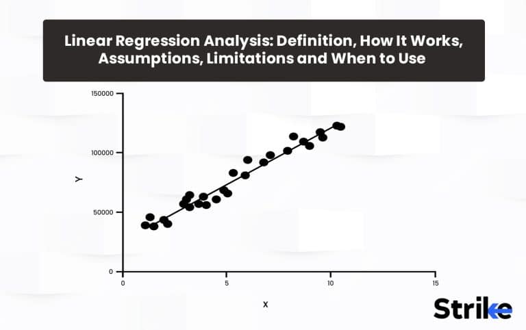
Linear Regression Analysis: Definition, How It Works, Assumptions, Limitations and When to Use

Linear regression analysis is a statistical technique for modeling linear relationships between variables. Linear regression is used to estimate real number values based on continuous data input. The goal here is to calculate an equation for a line that minimizes the distance between the observed data points and the fitted regression line. This line is then used to predict future values of the dependent variable based on new values of the independent variables.

For linear regression to work properly, assumptions about the data must be met. First, there must be a straight-line, linear relationship between the predictors and the response variable, with the change in response constant across the range of predictor values. Then, the residuals (errors between predicted and actual values) should be randomly distributed around a mean of zero, with no discernible patterns. Also, the residuals need to be independent from each other, so the value of one does not affect others. There should be no multicollinearity between the predictors, so each provides unique explanatory power as well. It is important that there should be no major outliers that skew the distribution. The residuals should follow a normal bell curve distribution here.

Linear regression does have limitations as well. It relies on simple linear models that cannot capture complex nonlinear relationships. Overfitting can occur with too many independent variables without proper regularization. It cannot directly model categorical predictors, only numeric continuous values. And confounding variables can distort results if not properly controlled for.

What Is Linear Regression Analysis?

Linear regression analysis is the data analysis technique that allows traders to predict unknown data by using data on a known value. The linear regression analysis can also be used in Stock markets to predict price movements as various variables meet at a common denominator.

The linear regression analysis is useful for short term traders and day traders as it gives key price points that can be used to place trades with appropriate risk management in consideration. These key price points offered by linear regression can be used to place buy, sell, stop loss and take profit orders. 

Linear regression analysis is formalized into a linear regression indicator that can be applied on charts to identify these key price points. The indicator is of two types, Linear regression curve and linear regression slope. Both of these indicators are different yet derived from the common theory of linear regression analysis. 

The Linear Regression Curve reflects or plots the predicted price movements at the end of specified number of bars or candles.

For example, a 14 period linear regression curve will equal the end value of a Linear Regression line that covers 14 candles. 

This linear regression curve may be beneficial on lower time frames for short term traders. The line is somewhat similar to moving averages.

Linear regression slope proceeds into positive and negative slopes. A positive of the curve indicates possibilities for upward movement in prices while a negative slope indicates possibilities for a downward momentum.

The slope oscillates between +100, +50 0 -50 and -100 levels. +100 and -100 are considered to be two extreme points from where the greater extent of reversals could be expected whereas crossing of the curve above or below 0 level indicates upward or downward momentum.

+50 and -50 levels are also potential swing points from where the slope may take turns and result in momentum shifts. The image uploaded below showcases both; the Linear Regression Curve and the Linear Regression Slope.

How Does Linear Regression Analysis Work?

Linear regression works by attempting to model the relationship between a dependent variable (Security’s price) and one or more independent variables (time) as a linear function. The overall goal is to derive a linear regression equation that minimizes the distance between the fitted line and the actual data points. This linear function allows estimating the value of the dependent variable based on the independent variables involved and thus helps in predicting the future price.

Linear regression analysis involves postulation of a linear relationship between a dependent variable such as security’s prices and independent variable such as time. The relationship between the two variables based on historical periods provides an opportunity to predict the future price.

A specific script is selected and the relationship between the dependent and independent variables are studied. It is observed that the historical price movement of the specific script’s price (dependent variable) reacts to time (independent variable) and the slope is formed. The positive slope formed between the variables refers to a directly proportional relationship between the two whereas a negative slope between the dependent and independent variables refers to an inverse relationship between the two. 

Broadly, Linear regression theory is used to create two indicators named; Linear regression curve and linear regression slope.

These indicators can be applied on a script’s chart to identify potential trade opportunities. 

Linear Regression Curve: 

The Linear Regression Curve is similar to a moving average but the linear regression curve has an edge over an ordinary moving average. The moving average plots an average of past price action whereas the linear regression curve plots where a linear regression line would expect the price of the script to be making the indicator more reactive and responsive than an ordinary moving average. 

The linear regression curve has a default time period setting set at 63. Although, time periods of 14 and 25 periods are also used. 

The image uploaded below shows an example of how 63 period linear regression curve can be used to take trades. A lower time period setting would be appropriate for short term trading whereas the 25 day setting is more useful for long term traders. By diving into lower time frames, the key prices provided by the curve would have given ample trading opportunities.

Two linear regression curves can be applied on the chart and the crossovers between the smaller period and higher period can be used to take long and short trades respectively. The crossover strategy with this indicator is not used widely as the latter, individual curve and the linear regression slope is used rather. The example of crossover is attached in the chart below.

Linear regression slope: 

The linear regression slope is an advanced momentum oscillator that is used by traders to determine the strength and direction of the trend. It is created out of the theory of linear regression analysis. The positive and negative slopes are used respectively to generate trading opportunities. Firstly, The slope oscillates between +50 and -50 levels. When the slope reaches these extreme zones, potential reversal takes shape.

Secondly, the 0 level is also used by traders to get a directional perspective of the script. If the value goes above 0 in positive territory it is assumed that the bullish momentum will get kicked in whereas if it oscillates below the 0 level in the negative territory, bearish momentum will take turn. Thirdly, the indicator does have -100 and +100 levels, but it rarely touches these extremes.

Chart below represents how the Linear Regression Slope causes price to react when it reaches the levels like +50, 0, -50. If the indicator reaches -50 level, it is often articulated as the market is in an oversold zone and may shift the momentum towards upside. The black horizontal line represents the 0 line and the 2 blue lines represent the +50 and -50 extreme points. If the price breaks crosses 0 in the positive zone, a bullish sentiment is kicked in whereas if the indicator crosses below the 0 level, a bearish momentum is triggered.

The indicators are lagging indicators therefore they should not be used as a standalone indicator. They must be combined with multi-time frame analysis, price action analysis and different indicators and tools should be used in conjunction to produce a robust trading plan with appropriate risk management in consideration.

How Does Linear Regression Analysis Generate Predictions Easily?

One of the key uses of linear regression models is to generate predictions for the dependent variable quickly and easily. 

The indicators are applied on charts to gain directional bias, strength of the trend and possible future sentiment of the market.

The linear regression slope and linear regression curve are two types of indicators that are built on the principle of Linear Regression theory. For a smaller time frame, linear regression curve is used for smaller time period settings. The indicator looks like a moving average but is more responsive than the moving average. This is one of the ways Linear Regression analysis generates predictions easily but of course the indicator is not advised to be used as a standalone indicator because it has potential to generate misleading signals in choppy markets.

Let’s look at an example of how the linear regression curve can be used to generate trades on smaller time frames. The chart uploaded below is a 15 min time frame chart of Nifty 50. The time period setting of the LRC indicator is 25 Period. The traders note the key price point reflected by the Linear Regression and dive further deep in 5 min or 3 min charts to take high probability trade setups. One can observe that the Linear Regression Curve (LRC) is more responsive than the moving averages thus it provides higher frequency of trades but the indicator is prone to generate misleading signals in choppy or ranging markets.

For long term traders and investors, Linear Regression Slope is advised to be used alongside multiple indicators to generate trading opportunities as the Linear Regression Slope oscillates between +25, 0 and -25 levels on lower time frames. Using the Linear Regression Slope on higher time frames generates predictions easily. Lets look at an example attached below. 

In the first chart, one can observe, the Linear Regression Slope does not reach +50 and -50 levels easily on lower time frames. The chart is a 15 min candlestick chart of Nifty 50. Thus traders consider crossing over and below the 0 level to generate trade ideas. As one can observe, if the slope indicated crossing over 0 level in the positive zone, the price managed to follow through and go up whereas if the slope crossed below the 0 level the price managed to undergo a bearish trajectory. The indicator like all is prone to generate misleading signals as well. Divergences can also be spotted between the price and indicator to produce trade ideas represented by the red arrow. Observe the black arrows and how the price reflects the indicator respectively.

The second image is a Daily time frame chart of Nifty 50. Observe on higher time frames like daily, the indicator does reach +50 and -50 levels to reflect overbought and oversold zones. An example is uncovered. The arrow represents how the linear regression slope generated a bullish reversal trade when it reached -50 level indicating a probable chance of bounce from the oversold zone.

This way the Linear Regression Analysis is used to predict the upcoming movements in the stock markets easily. But as no indicator generates 100% accurate signals, traders combine multi-time frame analysis, price action analysis, candlestick patterns and multiple indicators and tools are used in conjunction to generate robust trading opportunities. 

How Is Linear Regression Analysis Used in Predicting Stock Market Trends and Patterns?

Linear regression is commonly used in financial analysis and stock market prediction by modeling the relationship between stock prices and influencing factors like company performance, macroeconomic conditions, or technical indicators. Below are nine of the key ways linear regression models enable predicting stock market trends and patterns.

A simple linear regression model is sometimes developed with a stock’s price as the dependent variable and time as the independent variable. The linear relationship with time captures the overall trend in the stock’s price over a historical period. 

The regression line from this model provides predictions of where the stock price is headed based on the identified trend. This is sometimes used to forecast future price direction.

Regressing a stock price on a market benchmark like the Nifty 50 indexes its price movements to broader market trends. The regression coefficients quantify how sensitive the stock is to the index.

This allows predicting what the stock will do based on forecasted movements in the overall market. Stocks closely tied to the market are sometimes identified.

Fundamentals like sales, revenue, and earnings metrics are added as independent variables to relate a stock’s valuation to the company’s financial performance. 

The coefficients show how stock prices change in response to company results. Earnings forecasts can then drive stock price predictions.

Macro factors like interest rates, inflation, GDP growth, unemployment etc. are sometimes included as drivers of stock prices. 

This enables making predictions for how stock prices will respond as economic conditions change. Causal relationships with the economy are quantified.

Technical trading indicators like moving average crossovers, relative strength, price momentum, volatility, and trading volumes are sometimes predictive of price movements. 

Regression models can identify which technical signals are most predictive for a stock’s price. These indicators can then drive forecasts.

Regressing a group of stocks against each other identifies how they tend to move together based on common sector or industry exposures. This can predict patterns like one stock leading or lagging the others.

The regression coefficients quantify the exact relationships between the independent variables and stock prices. This helps precisely understand how various factors drive prices rather than vague intuitions.

Predictive abilities are sometimes evaluated by testing the models out-of-sample. This prevents overfitting and indicates how well the relationships will hold up for future prediction.

Linear regression is a useful statistical tool for modeling stock market outcomes. It enables identifying and quantifying the factors that are most predictive of future price movements and trends based on historical data. By incorporating relationships between stock prices and market, economic, and company factors, linear regression can improve the accuracy of stock market forecasts and provide valuable signals for investment decisions.

What Are the Assumptions of Linear Regression Analysis in Stock Market Forecasting?

Linear regression is a commonly used technique in stock market analysis and forecasting. However, there are assumptions that need to be met for linear regression models to provide valid, reliable predictions. The main assumptions include the below.

Linear Relationship

There is a straight-line, linear relationship between the dependent variable (stock price/return) and the independent variables (factors used for prediction). Nonlinear relationships require transformations.

Constant Variance of Residuals (Homoscedasticity)  

The variance of the residuals, or errors between predicted and actual values, should be constant at all values of the independent variables. Violating this can distort relationships and significance tests. Plotting residuals can check for homoscedasticity. Remedial measures like weighting or transformations help when this assumption is violated.

Independence of Residuals

Residuals should be independent and random.

Normal Distribution of Residuals

Residuals should follow a normal bell curve distribution. Violations can make inferences about statistical significance invalid. Non-normal residuals need transformations.

No Perfect Multicollinearity

Independent variables should not demonstrate perfect collinearity. This happens when one independent variable is a perfect linear function of others. It can cause model estimation problems. Checking correlation coefficients between independent variables can identify collinearity issues. Dropping redundant collinear variables helps. 

Correct Specification

The model should be properly specified with the appropriate functional form and all relevant variables included. Misspecification can cause bias in coefficient estimates. Plotting relationships, testing different models, and statistical specification tests can help identify model deficiencies.

No Measurement Error 

There should be no error in measuring or recording the independent variables. Measurement errors make estimates inconsistent and biased. Careful data collection and recording procedures reduces measurement errors.

Appropriate Use of Available Data

The sample data used to estimate the model should be representative of the population. It needs to properly cover the desired forecast period and target market. Insufficient or non-random sampling can lead to inaccurate or unstable coefficient estimates.

Coefficient Stability 

The relationships quantified by the model should be stable over the forecasting period rather than changing over time. Violations make the model unreliable for forecasting. Testing stability using rolling regressions on different time periods can help identify instability issues.

Model Fit

The linear regression model should have acceptable fit in explaining variation in the stock returns or prices, as measured by R-squared, F-test, etc. Poor model fit suggests important variables are missing or relationships are mis-specified. Additional diagnostics can help improve model fit.

Prediction Intervals

When making forecasts, prediction intervals should be calculated around the projected values to quantify the range of probable values. This incorporates the model’s inherent uncertainty.

Out-of-Sample Testing

The model should be validated on an out-of-sample dataset to test its ability to make accurate predictions before deployment. In-sample fit alone is insufficient.

Domain Knowledge Use

The relationships modeled should agree with practical domain knowledge of how the stock market works. Purely data-driven models may not work well for forecasting due to overfitting. Expert judgment should inform model development.

Simplicity

The model should be as simple as possible for reliable forecasting yet complex enough to capture key relationships. Overly complex models tend to have poor out-of-sample predictive performance.

Regular Re-estimation

Models should be re-estimated regularly using the most recent data to ensure they reflect the current state of the market. Markets evolve so models need updating.

Quantitative Validation

Predictive ability should be quantitatively assessed based on error metrics like MAP and RMSE, along with directional accuracy metrics like confusion matrices. These provide objective measures of forecast reliability.

Economic Significance

Relationships should make practical sense in terms of direction and magnitude based on financial and economic theory. Spurious correlations tend to break down for forecasting.  

Cautious Interpretation

Forecasts are estimates, not certainty. Caution is required when using models to make investment decisions or infer causal relationships from correlational models. All models are sometimes wrong.

Linear regression models for stock forecasting require assumptions related to relationships, residuals, specification, data, stability, fit, validation, theory, and interpretation. Checking and validating these assumptions is crucial to avoid generating misleading or inaccurate forecasts.

What Are the Limitations of Linear Regression Analysis in Stock Market Forecasting?

Linear regression  has some inherent limitations that constrain its effectiveness for predicting stock market behavior. Being aware of these limitations is important for proper application and realistic expectations.

Nonlinear Relationships

Stock market dynamics often involve nonlinearities that linear regression cannot capture. This includes saturation effects, step-changes, thresholds, and complex interactions. Transformations to linearize relationships do not always succeed. Nonlinear modeling techniques are required.

Correlation Not Causation

Linear regression quantifies correlations and cannot definitively determine causation. Some correlated driver variables do not cause stock price changes. This limits their predictive power if correlations break down in the future.

Data Mining and Overfitting

Fitting many candidate models and selecting the best historical fit often leads to overfitting. This produces models that fail to generalize to new data. Validation on out-of-sample data is essential to avoid this.

Spurious Correlations

Some correlations found in sample data simply occur by chance and have no meaningful explanatory relationship. These tend to weaken or disappear in future data. Distinguishing spurious correlations from persistent relationships is challenging.

Model Instability  

Periodic re-estimation using recent data is required, but this reduces sample size.

Data Errors

Input data errors and noise like data collection mistakes, data entry errors, etc. influence model coefficients and distort predictions. Identification and cleaning of anomalous data is important. 

Omitted Variables

Variables not included in the model that have explanatory power will get attributed to those that are included, resulting in inaccurate coefficients and distorted effects. Including all relevant variables is ideal but difficult.

Confounding Variables 

Important explanatory variables are omitted and happen to be correlated with variables that are included makes it difficult to isolate the true driver of stock prices. Confounding makes interpretation tricky.

Normality Assumption

Stock returns are often not perfectly normally distributed. Violating this assumption affects the validity of model inference and significance testing. Transformations are sometimes required.

Complex Interactions

Linear models do a poor job capturing complex multivariate interactions between variables. Higher order interaction effects are often present in stock markets.

Unstructured Data

Linear regression requires quantitative data inputs. Qualitative, unstructured data like news, investor sentiment, analyst opinions contain predictive information but cannot be directly used in linear regression models.

Few Independent Observations 

Time series data like stock prices violate the assumption of independent observations. Adjacent observations are correlated over time. This distorts model fitting and statistical tests. Time series techniques should be used.

Rare Events 

Extremely rare or unprecedented events cannot be predicted based on historical data alone. Historical modeling has limitations during financial crashes, pandemics, geopolitical crises, etc. Expert human judgment is crucial.

False Precision

Linear models imply a precision in stock market forecasts that is often not warranted. Prediction intervals should be used to quantify the uncertainty in forecasts rather than relying solely on point predictions.

Differences Across Stocks

Relationships tend to vary depending on the specific stock. It is difficult to develop generalizable models that apply reliably across a diverse set of stocks. Individual custom models may perform better.

Survivorship Bias

Models estimated on existing stock data suffer from survivorship bias. Companies that went bankrupt or got delisted are excluded, skewing the modeling.

Alternative Data Needs

Regression relies solely on quantitative data inputs. But other alternative data like earnings call transcripts, executive interviews, organizational changes contain valuable signals ignored by linear regression.

Model Degradation

Even if a model is sound when initially built, its performance degrades over time as markets evolve. Mechanisms to detect when a model is no longer working well are needed.

No model is a silver bullet. Linear regression should be combined with domain expertise, human judgment, and model robustness testing to enhance its usefulness for prediction.

When to Use Linear Regression?

Linear regression excels at quantifying historical linear relationships between stock prices/returns and potential driver variables like financial metrics, macro factors, technical indicators etc. The regression coefficients estimate the magnitude and direction of each variable’s relationship with the stock price/return, controlling for other factors. This reveals which variables have been most important historically.

Statistical tests assess the significance of the overall model and individual predictors. R-squared evaluates overall fit. This understanding of historical correlations and variable importance can guide trading strategies and investment decisions. The linear model is used to forecast expected returns based on current values of the predictor variables. The regression equation plugged with the latest input data generates predicted expected returns going forward. This works best when the true relationships are linear and the key drivers exhibit some persistence over time. Limitations arise when relationships are nonlinear or change substantially over time.

The two indicators produced out of the theory of linear regression; that are; Linear Regression Slope and Linear Regression Curve are used respectively to identify trading opportunities. The indicators are quite reliable but should not be used in isolation as they are prone to product misleading signals.

The indicators can independently be applied on candlestick charts to procure any information that may be crucial to understand the current market dynamics. The technical skills are quite improved and by combining multiple indicators, one can strengthen a trading plan. 

Regressing stock prices on market indexes models how closely the stock follows the overall market. This indexes the stock’s price to the benchmark. Industry and sector-based multi-stock models can identify groups of stocks that tend to move together and lead/lag each other. Macroeconomic models relate the stock market to the underlying economic conditions.

Fundamental stock valuation models relate prices to financial metrics like revenues, earnings, profit margins to quantify the underlying business value. Cross-sectional models estimate the typical relationships across a sample of stocks. Time series models focus on company-specific historical relationships. 

However, linear regression has limitations in stock market analysis. Relationships are often nonlinear due to thresholds and saturation effects. Structural changes over time like regime shifts can reduce model reliability. Expert human judgment is still crucial to supplement pure data-driven models. Causality cannot be definitively established with correlations alone.

How Does Linear Regression Analysis Help Portfolio Optimization and Risk Management?

Regression models quantify the historical risk and return characteristics of each asset class based on historical data. This provides inputs for mean-variance portfolio optimization models to determine optimal asset allocation mixes. Factors like volatility, skew, tail risks, and drawdowns are modeled for downside risk.

The correlations between asset classes are modeled using regression to determine diversification benefits. Low correlation pairs are identified for combining into portfolios to improve the risk-return tradeoff. Regression also models lead-lag relationships between asset classes.

For a given portfolio, regressing individual stock returns on factors like market returns estimates each stock’s market beta. Stocks with higher betas are assigned smaller portfolio weights to manage overall portfolio risk exposure. Weights also be scaled lower for stocks with higher idiosyncratic volatility based on regression models.

Regressing asset returns on macroeconomic indicators  model how return patterns change across economic regimes like expansion vs recession. This allows tilting portfolios proactively towards assets poised to do well in an impending regime.

The indicators, linear regression slope and curve are utilized to validate a trading idea. Trap trades can be avoided by applying the indicator on the price chart. Possible higher risk:reward ratios can also be achieved by watching price action closely with the indicators applied. 

This way, if the indicators are used alongside multi-time frame analysis, price action, candlestick patterns and different indicators, a robust risk management module can be achieved. 

Regression models estimate the fair value for each asset based on fundamental drivers. Observing large residuals reveals assets trading significantly above or below fair value. This identifies potential buying or selling opportunities. Momentum and mean reversion tendencies are also modeled to optimize timing of trades.

Left tail risks be modeled by regressing drawdowns, volatility spikes, skew, kurtosis etc on market and macro factors. This quantifies how severely each asset gets impacted under large market sell-offs. Assets with less downside risk are overweight. 

The sensitivity of each asset to risk factors like interest rates and currencies can be modeled with regression. This determines appropriate hedging positions using derivatives like swaps, futures, and options to mitigate risks.

Regressing asset returns on factors like volatility and sentiment helps identify conditions predictive of impending drawdowns or crashes. Portfolios reduce risk preemptively based on these indicators before crashes materialize.

However, linear models do have limitations. Relationships between asset classes are often nonlinear. Structural breaks like policy regime shifts happen. Rare tail events are hard to model.

What Are the Common Variables and Factors Used in Linear Regression Analysis for Stock Market Investments?

The dependent variable in stock market regression is usually the stock return, which is measured in different ways such as raw return, excess return over a benchmark, or risk-adjusted return. The independent variables are the factors that are hypothesized to impact stock returns. Below are the most commonly used independent variables in stock market regression models.

Market Risk Factors

Market Return: The overall stock market return is one of the most fundamental factors driving individual stock returns. The market return is often represented by a broad market index such as the Nifty 50. Adding the market return as a factor accounts for the general correlation between a stock and the overall market.

Size Factor: The size factor (also called size premium) accounts for the empirical observation that small-cap stocks tend to outperform large-cap stocks in the long run. This factor is captured by sorting stocks into quintiles by market capitalization and going long small-cap stocks and short large-cap stocks. 

Value Factor: The value factor is based on the finding that stocks with low valuation multiples like price-to-earnings tend to deliver higher returns than growth stocks with high valuation multiples. This factor is captured by sorting stocks into value and growth buckets based on valuation ratios.

Momentum Factor: The momentum factor aims to capture the short-term persistence in stock returns. Stocks that have performed well recently tend to continue to outperform in the near future. This factor is implemented by going long recent winner stocks and short recent loser stocks.

Macroeconomic Variables 

GDP growth: The overall economic growth as measured by GDP growth rate has a significant impact on corporate earnings and thus stock returns. Including GDP growth accounts for the state of the overall economy.

Interest rates: Interest rates impact the rate at which future cash flows are discounted. Lower interest rates tend to boost stock valuations.

Inflation: Inflation erodes the real purchasing power of future corporate earnings and dividends. Adding inflation adjusted stock returns for loss of purchasing power. The Consumer Price Index (CPI) is used to measure inflation.

Industrial production: The monthly change in industrial production indexes the growth of the manufacturing sector and the real economy. It serves as an indicator for the business cycle. 

Unemployment rate: The unemployment rate measures slack in the labor market. A lower unemployment rate indicates a strong economy and labor market.

Oil prices: As a key input cost for many companies, the price of oil impacts the earnings outlook for several sectors and thus broader stock market performance. The WTI crude oil spot price is used for oil price fluctuations.

Sector and Industry Factors

Sector returns: Rather than the broad market return, sector-specific returns are added to control for industry-level trends. The regression includes returns for each sector such as energy, materials, industrials, consumer discretionary, staples, healthcare, financials, information technology, communication services, utilities, and real estate.

Industry classification: Industry dummy variables divide stocks into different groups based on their industry classification such as technology, energy, consumer goods, healthcare etc. This controls for divergence in performance between different industries.

Commodity prices: For commodity producers, commodity prices are a significant driver of revenues and profits. Relevant commodity prices like copper, aluminum etc. are added for those sectors.

Company-Specific Factors 

Earnings yield: The inverse of the price-to-earnings ratio serves as a valuation-based factor. High earnings yield stocks have tended to outperform the market. 

Book-to-market: The book value to market capitalization ratio has been shown to predict returns. Stocks with high book-to-market ratios have delivered superior returns historically.

Sales growth: Earnings ultimately follow from sales, so past sales growth signal future earnings growth potential. Trailing 12-month or 3-year sales growth is used.

Return on equity: Return on equity measures profitability. Stocks with high returns on equity have seen better stock returns. 

Momentum: Trailing 6-month or 12-month returns capture stock price momentum, which persists in the short run. 

Earnings surprise: The most recent earnings surprise relative to analyst estimates captures near-term sentiment around a company.

In addition to the above fundamental factors, regression models also incorporate technical indicators like moving average crossovers, breakouts, price-volume trends etc. as independent variables. 

The regression is estimated across all stocks in the market, within specific sectors/industries, or at the individual stock level. The time frame of the data used also varies; shorter windows like 1-year are common for near-term forecasting while much longer multi-decade histories are used to evaluate factor performance. 

Stock return as the dependent variable and a combination of the above independent variables, the regression gives the sensitivity of the stock to each factor (the coefficients) as well as the statistical significance. It then is used to forecast expected returns based on current values of the explanatory variables. Evaluating the coefficient of determination R-squared shows how much of the variation in stock returns is explained by the regression model.

What Are the Different Types of Linear Regression Models Used in Stock Market Analysis?

Simple linear regression involves one independent variable and is used to model the relationship between a stock’s returns and a single factor such as the market return or a specific risk factor.

Multiple linear regression includes multiple independent variables and allows modeling stock returns based on a combination of factors like valuation ratios, macroeconomic indicators, industry performance, and other variables.

Simple linear regression is used to model the relationship between two variables – a dependent variable and a single independent or explanatory variable. It tries to fit a linear equation to observed data points in order to predict the dependent variable from the independent variable. 

In stock market analysis, simple linear regression is commonly used to examine the influence of a single factor on stock returns. For example, you could use it to understand how monthly returns of an individual stock are affected by the monthly returns of a broad market index like the Nifty 50.

2. Multiple Linear Regression

Multiple linear regression allows simultaneously modeling the impact of multiple independent variables. This provides a more comprehensive analysis by accounting for different drivers of stock returns beyond just the market.

Key benefits of multiple regression are accounting for multiple return drivers and quantifying the impact of different variables. But a limitation is avoiding overfitting by not including too many insignificant variables in the model. Feature selection techniques are used to determine the optimal set of factors that maximizes explanatory power without overfitting.

How Does Multicollinearity Impact Linear Regression Analysis in The Stock Market?

Multicollinearity refers to a situation where two or more explanatory variables in a multiple regression model are highly correlated with each other. This poses problems when interpreting the results and performance of linear regression models for stock market analysis.

Independent variables are highly correlated means it becomes difficult to separate out the individual effect of each variable on the dependent variable (stock returns). The coefficients of collinear variables are unstable and difficult to estimate precisely. Slight changes in the data lead to wide swings in the coefficient estimates.

For example, valuation ratios like the price-to-earnings (P/E) ratio and price-to-book (P/B) ratio often demonstrate high correlation. Including both in a regression model does not always  provide accurate insights into the isolated influence of each ratio on stock returns. 

High multicollinearity also inflates the standard errors of coefficient estimates. This makes it harder to determine if coefficients are statistically significant. Collinear variables show up as insignificant even if jointly they have strong explanatory power.

In the presence of multicollinearity, the overall fit of the model appears sound based on a high R-squared value. But the estimates of individual coefficient values and statistical tests are unreliable. So multicollinearity reduces the predictive accuracy of a model even though the overall fit looks good.

There are a few common remedies for multicollinearity in stock market regression analysis.

Removing highly correlated variables 

Keep only one of the collinear variables most relevant based on economic logic and research. For example, just use the P/B ratio instead of both P/B and P/E.

Obtaining more data 

A larger data sample helps improve coefficient estimation for collinear variables.

Applying regularization 

Techniques like ridge regression and LASSO add a penalty term to shrink unstable coefficient estimates towards zero. 

Using principal components analysis Instead of correlated variables, principal components are used as regressors. These are linear combinations of the variables that are orthogonal and uncorrelated.

Leveraging economic logic Rely on economic theory to guide interpretation of coefficients on correlated variables instead of purely statistical estimates.

Multicollinearity is not necessarily a major problem if the regression’s purpose is forecasting stock returns. The model still   manages to predict reasonably well out of sample. But it does require careful handling of coefficient estimates and statistical inference.

How Can Outliers Affect the Results of Linear Regression Analysis in Stock Market Forecasting?

Outliers refer to data points that are abnormally far away from the majority of observations. They skew and distort the results of linear regression models used for stock return forecasting.

Outliers arise in stock market data for several reasons like temporary volatility spikes, data errors, or extreme events. For example, a stock price crashing during a market crash recession could appear as an outlier relative to its normal range of returns.

Including outliers when fitting a linear regression model significantly drags the regression line towards those extreme points. This reduces the precision of the model in representing the typical relationship between variables for most observations.

The slope of the regression line becomes more tilted due to outlier data points with high leverage. This distorts the magnitude of the coefficients which represent the relationships between variables. The intercept also gets pulled towards outliers.

As a result, predictions made by the regression equation become less accurate for most data points except the outliers. Forecasts tend to be skewed and oversensitive to the outliers.

For example, a high inflation reading from the 1980s crisis sometimes causes a stock return regression model to overestimate the impact of inflation. Predictions would be distorted for normal inflation ranges based on this temporary historical anomaly.

Outliers also increase the variability and decrease the overall model fit. The R-squared decreases as outliers are not well represented by the model. Standard errors rise as well. This reduces the reliability of coefficient estimates.

Can I Generate Linear Regression Analysis in Excel?

Yes, performing linear regression analysis in Excel is straightforward using the built-in Data Analysis Toolpak. Here is a quick overview of the process:

First, activate the Data Analysis Toolpak add-in if it is not already enabled. Go to File > Options > Add-ins and manage Excel add-ins to turn on Analysis Toolpak.

Next, organize your data with the dependent variable (y) in one column and independent variable(s) (x) in adjacent columns. The data should not contain any empty cells. Label the columns appropriately.

Then go to the Data tab in the toolbar and click Data Analysis. In the popup window, select Regression from the list and click OK. 

In the Regression dialog box, input the y and x ranges. Check the appropriate options for labels, confidence intervals, etc. Click OK and Excel will output a results table on a new worksheet with the regression statistics including coefficients, R-squared, standard errors, t-stats, and p-values.

The built-in Excel regression tool makes it easy to quickly analyze and visualize linear relationships between variables. The results are used to predict the dependent variable from the independent variables based on the calculated equation.

Can I Generate Linear Regression Analysis on Mat Lab?

Yes, MATLAB provides comprehensive tools for performing linear regression analysis. The Statistics and Machine Learning ToolboxTM in MATLAB includes functions like fitlm, stepwiselm, lasso, ridge, and many others for fitting linear models.

Is Linear Regression Used to Identify Key Price Points, Entry Prices, Stop-Loss Prices, and Exit Prices?

Yes, linear regression is used in financial analysis to identify important price levels. By modeling the relationship between price and volume, time, or other factors, the indicators are produced from the theory itself such as Linear Regression Slope and Linear Regression Curve, that are applied on charts to gain important key price points, regression can determine price points that act as support or resistance as well as project future values. These price levels can serve as potential entry, stop loss or exit points for trades. However, sound trading strategies would combine regression with other indicators rather than rely solely on it.

Arjun Remesh

Head of Content

Arjun is a seasoned stock market content expert with over 7 years of experience in stock market, technical & fundamental analysis. Since 2020, he has been a key contributor to Strike platform. Arjun is an active stock market investor with his in-depth stock market analysis knowledge. Arjun is also an certified stock market researcher from Indiacharts, mentored by Rohit Srivastava.

Shivam Gaba

Reviewer of Content

Shivam is a stock market content expert with CFTe certification. He is been trading from last 8 years in indian stock market. He has a vast knowledge in technical analysis, financial market education, product management, risk assessment, derivatives trading & market Research. He won Zerodha 60-Day Challenge thrice in a row. He is being mentored by Rohit Srivastava, Indiacharts.